Many systems are configured using JSON (or YAML), and there is often a need to parameterize such configuration. Examples include: AWS CloudFormation, Terraform, Google Cloud Deployment Manager, Taskcluster Tasks/Hooks, the list goes on.
This paramterization is usually accomplished with one of the following approaches:
Use of custom variable injection syntax and special rules,
Rendering with a string templating engine like jinja2 or mustache prior to parsing the JSON or YAML configuration, or,
Use of a general purpose programming language to generate the configuration.
Approach (1) is for example used by AWS CloudFormation and Terraform. In Terraform variables can be injected with string interpolation syntax, e.g. ${var.my_variable}, and resource objects with a count = N property are cloned N times. Drawbacks of this is that each system have its own logic and rules that you’ll have to learn. Often these are obscure, verbose and/or inconsistent, as template language design isn’t the main focus of a project like Terraform or CloudFormation.
Approach (2) is among other places used in Google Cloud Deployment Manager, it was also employed in earlier versions of .taskcluster.yml. For example in Google Cloud Deployment Manager your infrastructure configuration file is rendered using jinja2 before being parsed as YAML. Which allows you to make a parameterized infrastructure configuration. While this approach reuse existing template logic, drawbacks include the fact that after passing through the text template engine your JSON or YAML may no longer parse due to whitespace issues, commas or other terminals accidentally injected. If the template is big, this is easy to do, resulting in errors that are hard to understand and track down.
Approach (3) is for example used by vagrant where config files are written in Ruby. It’s also used in gecko where moz.build files written in Python define which source files to compile. This approach is powerful, and reuse existing established languages. Drawbacks of this approach is that you need sandboxing to read untrusted config files. This approach also binds you to a specific programming language, or at-least forces you to have an interpreter for said language installed. Finally, there can be cases where these, often imperative configuration files becomes clutter and littered with if-statements.
Introducing json-e
json-e is a language for parameterization of JSON following approach (1), which is to say you can write your json-e template as JSON, YAML or anything that translates to a JSON object structure in-memory. Then the JSON structure can be rendered with json-e, meaning interpolation of variables and evaluation of special constructs.
An example is probably the best way to understand json-e, below is a javascript example of how json-e works.
Most of the variable interpolation here is obvious, but constructs like {$if: E, then: A, else: B} are very powerful. Here E is an expression while A and B are templates. Depending on the expression the whole construct is replaced with either A or B, if either one of those are omitted the parent property or array index is deleted.
As evident from the example above json-e contains an entire expression language. This allows for complex conditional constructs and powerful variable injection. Aside from the expression language json-e defines a set of constructs. These are objects containing a special keyword property that always starts with $. The conditional $if is one such construct. These constructs allows for evaluation of expressions, flattening of lists, merging of objects, mapping elements in a list and many other things.
The constructs are first interpreted after JSON parsing. Hence, you can write json-e as YAML and store it as JSON. In fact, I would recommend writing json-e using YAML as this is very elegant. For a full reference of all the constructs, built-in functions, and expression language features checkout the json-e documentation site, it even includes an interactive json-e demo tool.
Design Choices
Unlike the special constructs and syntax used in AWS CloudFormation and Terraform, json-e aim to be a general purpose JSON parameterization engine. So ideally, json-e can be reused in other projects. The design is largely guided by the following desires:
Familiarity to Python and Javascript developers,
Injection of variables after parsing JSON/YAML,
Safe rendering without need for OS-level sandboxing,
Extensibility by injection of functions as well as variables,
Avoid Turing completeness to prevent templates from looping forever,
Side-effect free results (baring side-effects in injected functions),
Implementation in multiple languages.
We wanted safe rendering because it allows for services like taskcluster-github to render untrusted templates from .taskcluster.yml files. Similarly, we wanted implementations in multiple languages to avoid being tied to specific programming language, but also to facilitate web-based tools for debugging json-e templates.
State of json-e Today
As of writing the json-e repository contains and implementation of json-e in Javascript, Python and golang, along with a large set of test cases to ensure compatibility between the implementations. Writing a json-e implementation is fairly straight forward, so new implementations are likely to show up in the future.
For those interested in the details I recommend reading about Pratt-parsers, which have made implementation of the same interpreter in 3 languages fairly easy.
Today, json-e is already used in-tree (in gecko), we use it as part of the interface for expressing actions and be triggered in the automation UI. For those interested there is the in-tree documentation and the actions.json specification. We also have plans to use json-e for a few other things including github integration and taskcluster-hooks.
As for stability we may add new construct and functions json-e in the future, but major changes are not planned. For obvious reasons we don’t want to break backwards compatibility, this have happened a few times initially, mostly to correct things that were unintended design flaws. We still have a few open issues like unicode handling during string slicing. But by now we consider json-e stable.
On a final note I would like to extend a huge thanks to the many contributors who have worked on json-e, as of writing the github repository already have commits from 12 authors.
Last summer Edgar Chen (air.mozilla.org) built on an interactive shell for TaskCluster Linux workers, so developers can get a SSH-like session into a task container from their browser. We’ve slowly been improving this, and prior to Mozlando I added support for opening a VNC-like session connecting to an X-session inside a task container. I’ll admit I was mostly motivated by the prospect of giving an impressive demo, and the implementation details are likely to change as we improve it further. Consequently, we haven’t got many guides on how to use these features in their current state.
However, with people asking for TaskCluster “loaners” on IRC, I figure now is a good time to explain how these interactive features can be used to provide a loaner-on-demand flow for TaskCluster workers. At least on Linux, but hopefully we can do a similar thing on other platforms too. Before we dive in, I want to note that all of our Linux tasks runs under docker with one container per tasks. Hence, you can pull down the docker image and play with it locally, the process and caveats such as setting up loopback video and audio devices is beyond the scope of this post. But feel free to ask on IRC (#taskcluster), I’m sure Greg Arndt has all the details, some of them are already present in “Run Locally” script displayed in the task-inspector.
Quick Start
If you can’t wait to play, here are the bullet points:
You’ll need a commit-level 1 access (and LDAP login)
Under “Job details” click the “Inspect Task” (this will open the task-inspector)
In the top right corner in the task-inspector click “Login” (this opens login.taskcluster.net on a new tab)
“Sign-in with LDAP” or “Sign-in with Okta” (Okta only works for employees)
Click the “Grant Access” button (to grant tools.taskcluster.net access)
In the task-inspector under the “Task” tab, scroll down and click the “One-Click Loaner” button
Click again to confirm and create a one-click loaner task (this takes you to a “Waiting for Loaner” page)
Just wait… 30s to 5 min (you can open the task-inspector for your loaner task to see the live log, if you are impatient)
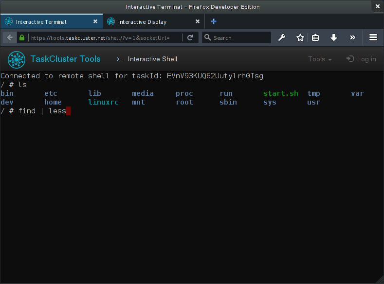
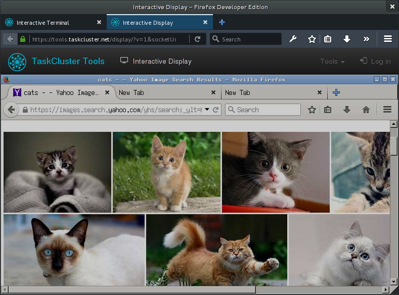
Eventually you should see two big buttons to open an interactive shell or display
You should now have an interactive terminal (and display) into a running task container.
Warning: These loaners runs on EC2 spot-nodes, they may disappear at any time. Use them for quickly trying something, not for writing patches.
Given all these steps, in particular the “Click again” in step (6), I recognize that it might take more than one click to get a “One-Click Loaner”. But we are just getting started, and all of this should be considered a moving target. The instructions above can also be found on MDN, where we will try to keep them up to date.
Implementation Details
To support interactive shell sessions the worker has an end-point that accepts websocket connections. For each new websocket the worker spawns a sh or bash inside the task container and pipes stdin, stdout and stderr over the websocket. In browser we use then have the websocket reading from and writing to hterm (from the chromium project) giving us a nice terminal emulator in the browser. There is still a few issues with the TTY emulation in docker, but it works reasonably for small things.
For interactive display sessions (VNC-like sessions in the browser) the worker has an end-point which accepts both websocket connections and ordinary GET requests for listing displays. For each GET request the worker will run a small statically linked binary that lists all the X-sessions inside the task container, the result is then transformed to JSON and returned in the request. Once the user has picked a display, a websocket connection is opened with the display identifier in query-string. On the worker the websocket is piped to a statically linked instance of x11vnc running inside the task container. In the browser we then use noVNC to give the user an interactive remote display right in the browser.
As with the shell, there is also a few quirks to the interactive display. Some graphical artifacts and other “interesting” issues. When streaming a TCP connection over a websocket we might not be handling buffering all too well. Which I suspect introduces additional latency and possible bugs. I hope these things will get better in future iterations of the worker, which is currently undergoing an experimental rewrite from node to go.
Future Work
As mentioned in the “Quick Start” section, all of this is still a bit of a moving target. Access is to any loaner is effectively granted to anyone with commit level 1 or any employee. So your friends can technically hijack the interactive task you created. Obviously, we have to make that more fine-grained. At the moment, the “one-click loaner” button is also very specific to our Linux worker. As we add more platforms will have to extend support and find a way to abstract the platform dependent aspects. S it’s very likely that this will break on occasion.
We also recently introduced a hack defining the environment variable TASKCLUSTER_INTERACTIVE when a loaner task is created. A quick hack that we might refactor later, but for now it’s enabling Armen Zambrano to customize how the docker image used for tests runs in loaner-mode. In bug 1250904 there is on-going work to ensure that a loaner will setup the test environment, but not start running tests until a user connects and types the right command. I’m sure there are many other things we can do to make the task environment more useful in loaner-mode, but this is certainly a good start.
Anyways, much of this is still quick hacks, with rough edges that needs to be resolved. So don’t be surprised if it breaks while we improve stability and attempt to add support for multiple platforms. With a bit of time and resources I’m fairly confident that the “one-click loaner” flow could become the preferred method for debugging issues specific to the test environment.
When we started building TaskCluster about a year and a half ago one of the primary goals was to provide a self-serve experience, so people could experiment and automate things without waiting for someone else to deploy new configuration. Greg Arndt (:garndt) recently wrote a blog post demystifying in-tree TaskCluster scheduling. The in-tree configuration allows developers to write new CI tasks to run on TaskCluster, and test these new tasks on try before landing them like any other patch.
This way of developing test and build tasks by adding in-tree configuration in a patch is very powerful, and it allows anyone with try access to experiment with configuration for much of our CI pipeline in a self-serve manner. However, not all tools are best triggered from a post-commit-hook, instead it might be preferable to have direct API access when:
Locating existing builds in our task index,
Debugging for intermittent issues by running a specific task repeatedly, and
Running tools for bisecting commits.
To facilitate tools like this TaskCluster offers a series of well-documented REST APIs that can be access with either permanent or temporary TaskCluster credentials. We also provide client libraries for Javascript (node/browser), Python, Go and Java. However, being that TaskCluster is a loosely coupled set of distributed components it is not always trivial to figure out how to piece together the different APIs and features. To make these things more approachable I’ve started a series of interactive tutorials:
All these tutorials are interactive, featuring a runtime that will transpile your code with babel.js before running it in the browser. The runtime environment also exposes the require function from a browserify bundle containing some of my favorite npm modules, making the example editors a great place to test code snippets using taskcluster or related services.
As part of my goals this quarter I’ve been experimenting with running Talos in the cloud (Linux only). There are many valid reasons why we’re not already doing this. Conventional wisdom dictates that visualized resources running on hardware shared between multiple users is unlikely to have consistent performance profile, hence, regressions detection becomes unreliable.
Another reason for not running performances tests in the cloud, is that a cloud server is very different from a consumer laptop, and changes in performance characteristic may not reflect the end-user experience.
But when all the reasons for not running performance testing in the cloud have been listed, and I’m sure my list above wasn’t exhaustive. There certainly is some benefits to using the cloud, on-demand scalability and cost immediately springs to mind. So investigating the possibility of running Talos in the cloud is interesting, if not thing more it could be used for fast smoke tests.
Comparing Consistency of Instance Types
First thing to evaluate is the consistency of results depending on instance-type, cloud provider and configuration. For the purpose of these experiments I have chosen instances and cloud providers:
Digital Ocean (1g-1cpu, 2g-2cpu, 4g-2cpu, 8g-4cpu)
For AWS I tested instances in both us-east-1 and us-west-1 to see if there was any difference of results. In each case I have been using two revisions c448634fb6c9 which doesn’t have any regressions and fe5c25b8b675 which has clear regressions in test suites cart and tart. In each case I also ran the tests with both xvfb and xorg configured with dummy video and input drivers.
To ease deployment and ensure that I was using the exact same binaries across all instances I packaged Talos as a docker image. This also ensured that I could reset the test environment after each Talos invocation. Talos was invoked to run as many of the test suites as I could get working, but for the purpose of this evaluation I’m only considering results from the following suites:
tp5o,
tart,
cart,
tsvgr_opacity,
tsvgx,
tscrollx,
tp5o_scroll, and
tresize
After running all these test suites for all the configurations of instance type, region and display server enumerated above, we have a lot of data-points on the form results(cfg, rev, case) = (r1, r2, ..., rn), where ri is the measurement from the i’th iteration of the Talos test case case.
To compare all this data with the aim of ranking configurations by the consistency of their results, compute rank(cfg, rev, case) as the number of configurations cfg' where rank(cfg', rev, case) < rank(cfg, rev, case). Informally, we sort configurations based lowest standard deviation for a given case and rev and the index of a configuration in that list is the rank rank(cfg, rev, case) of the configuration for the given case and rev.
We then finally list configurations by score(cfg), which we compute as the mean of all ranks for the given configuration. Formally we write:
score(cfg) = mean({rank(cfg, rev, case) | for all rev, case})
Credits for this methodology goes to Roberto Vitillo, who also suggested using trimmed mean, but as it turns out the ordering is pretty much the same.
When listing configurations by score as computed above we get the following ordered lists of configurations. Notice that the score is strictly relative and doesn’t really say much. The interesting aspect is the ordering.
Warning, the score and ordering has nothing to do with performance. This strictly considers consistency of performance from a Talos perspective. This is not a comparison of cloud performance!
You may notice that the list above also contains the configuration mozilla-inbound-non-pgo which has results from our existing infrastructure. It is interesting to see that instances with high CPU exhibits lower standard deviation. This could be because their average run-time is lower, so the standard deviation is also lower. It could also be because they consist of more high-end hardware, SSD disks, etc. Higher CPU instances could also be producing better results because they always have CPU time available.
However, it’s interesting that both Azure and Digital Ocean instances appears to produce much less consistent results. Even their high-performance instances. Surprisingly, the data from mozilla-inbound (our existing infrastructure) doesn’t appear to be very consistent. Granted that could just be a bad run, we would need to try more revisions to say anything conclusive about that.
Unsurprisingly, it doesn’t really seem to matter what AWS region we use, which is nice because it just makes our lives that much simpler. Nor does the choice between xorg or xvfb seem to have any effect.
Comparing Consistency Between Instances
Having identified the Amazon c4 and c3 instance-types, as the most consistent classes, we now proceed to investigate if results are consistent when they are computed using difference instances of the same type. It’s well known that EC2 has bad apples (individual machines that perform badly), but this is a natural thing in any large setting. What we are interested in here is what happens when we compare results different instances.
To do this we take the two revisions c448634fb6c9 which doesn’t have any regressions and fe5c25b8b675 which does have a regression in cart and tart. We run Talos tests for both revisions on 30 instances of the same type. For this test I’ve limited the instance-types under consideration to c4.large and c3.large.
After running the tests we now have results on the form results(cfg, inst, rev, suite, case) = (r1, r2, ... rn) where ri is the result from the i’th iteration of the given test case under the given test suite, revision, configuration and instance. In the previous section we didn’t care which suite the test case belonged to. We care about suite relationship here because we compute the geometric mean of the medians of all test cases per suite. Formally we write:
score(cfg, inst, rev, suite) = geometricMean({median(results(cfg, inst, rev, suite, case)) | for all case})
Credits to Joel Maher for helping figure out how the current infrastructure derives per suite performance score for a given revision.
We then plot the scores for all instances as two bar-chart series one for each revision. We get the following plots. I’ve only included 3 here for brevity. Each pair of bars is results from one instance on different revisions, the ordering here is not relevant.
From these two plots it’s easy to see that there is a there is a tart regression. Clearly we can also see that performance characteristics does vary between instances. Even in the case of tart it’s evident, but it’s still easy to see the regression.
Now when we consider the chart for tresize it’s very clear that performance is different between machines. And if a regression here was small, it would be hard to see. Most of the other charts are somewhat similar, I’ve posted a link to all of them below along with references to the very sketchy scripts and hacks I’ve employed to run these tests.
While it’s hard to conclude anything definitive without more data. It seems that the C4 and C3 instance-types offers fairly consistent result. I think the next step is to setup a subset of Talos tests running silently along side existing tests while comparing results to regressions observed elsewhere.
Hopefully it should be possible to use a small subset of Talos tests to detect some regressions early. Rather than having all Talos regressions detected 12 pushes later. Setting this up is not going to a Q2 goal for me, but I should be able to set it up on TaskCluster in no time. At this point I think it’s mostly a configuration issue, since I already have Talos running under docker.
The hard part is analyzing the resulting data and detect regressions based on it. I tried comparing results with approaches like students t-tests. But there is still noisy tests that have to be filtered out, although preliminary findings were promising. I suspect it might be easiest to employ some naive form of Machine learning, and hope that magically solves everything. But we might not have enough training data.
When I was working on the aggregation code for telemetry histograms as displayed on the telemetry dashboard, I also wrote a Javascript library (telemetry.js) to access the aggregated histograms presented in the dashboard. The idea was separate concerns and simplify access to the aggregated histogram data, but also to allow others to write custom dashboards presenting this data in different ways. Since then two custom dashboards have appeared:
Both of these dashboards runs a cronjob that downloads the aggregated histogram data using telemetry.js and then aggregates or analyses it in an interesting way before publishing the results on the custom dashboard. However, telemetry.js was written to be included from telemetry.mozilla.org/v1/telemetry.js, so that we could update the storage format, use a differnet data service, move to a bucket in another region, etc. I still want to maintain the ability to modify telemetry.js without breaking all the deployments, so I decided to write a node.js module called telemetry-js-node that loads telemetry.js from telemetry.mozilla.org/v1/telemetry.js. As evident from the example below, this module is straight forward to use, and exhibits full compatibility with telemetry.js for better and worse.
// Include telemetry.jsvar Telemetry =require('telemetry-js-node');// Initialize telemetry.js just the documentation says to
Telemetry.init(function(){// Get all versionsvar versions = Telemetry.versions();// Pick a versionvar version = versions[0];// Load measures for version
Telemetry.measures(version,function(measures){// Print measures available
console.log("Measures available for "+ version);// List measures
Object.keys(measures).forEach(function(measure){
console.log(measure);});});});
Whilst there certainly is some valid concerns (and risks) with loading Javascript code over http. This hack allows us to offer a stable API and minimize maintenance for people consuming the telemetry histogram aggregates. And as we’re reusing the existing code the extensive documentation for telemetry is still applicable. See the following links for further details.
Disclaimer: I know it’s not smart to load Javascript code into node.js over http. It’s mostly a security issue as you can’t use telemetry.js without internet access anyway. But considering that most people will run this as an isolated cron job (using docker, lxc, heroku or an isolated EC2 instance), this seems like an acceptable solution.
By the way, if you make a custom telemetry dashboard, whether it’s using telemetry.js in the browser or Node.js, please file a pull request against telemetry-dashboard on github to have a link for your dashboard included on telemetry.mozilla.org.
In the past quarter I’ve been working on analysis of telemetry pings for the telemetry dashboard, I previously outlined the analysis architecture here. Since then I’ve fixed bugs, ported scripts to C++, fixed more bugs and given the telemetry-dashboard a better user-interface with more features. There’s probably still a few bugs around, decent logging is still missing, but data aggregated is fairly stable and I don’t think we’re going to make major API changes anytime soon.
So I think it’s time to let others consume the aggregated histograms, enabling the creation of custom dashboard. In the following sections I’ll demonstrate how to get started with telemetry.js and build a custom filtered dashboard with CSV export.
Getting Started with telemetry.js
On the server-side the aggregated histograms for a given channel, version and measure is stored in a single JSON file. To reduce storage overhead we use a few tricks, such as translating filter-paths to identifiers, appending statistical fields at the end of a histogram array and computing bucket offsets from specification. This makes the server-side JSON files rather hard to read. Furthermore, we would like the flexibility to change this format, move files to a different server or perhaps do a binary encoding of histograms. To facilitate this, data access is separated from data storage with telemetry.js. This is a Javascript library to be included from telemetry.mozilla.org/v1/telemetry.js. We promise that best efforts will be made to ensure API compatibility of the telemetry.js version hosted at telemetry.mozilla.org.
I’ve used telemetry.js to create the primary dashboard hosted at telemetry.mozilla.org, so the API grants access to the data used here. I ‘ve also written extensive documentation for telemetry.js. To get you started consuming the aggregates presented on the telemetry dashboard, I’ve posted the snippet below to a jsfiddle. The code initializes telemetry.js, then proceeds load the evolution of a measure over build dates. Once loaded the code prints a histogram for each build date of the 'CYCLE_COLLECTOR' measure within 'nightly/27'. Feel free to give it a try…
Telemetry.init(function(){
Telemetry.loadEvolutionOverBuilds('nightly/28',// from Telemetry.versions()'CYCLE_COLLECTOR',// From Telemetry.measures('nightly/28', callback)function(histogramEvolution){
histogramEvolution.each(function(date, histogram){print("--------------------------------");print("Date: "+ date);print("Submissions: "+ histogram.submissions());
histogram.each(function(count, start, end){print(count +" hits between "+ start +" and "+ end);});});});});
Warning: the channel/version string and measure string shouldn’t be hardcoded. The list of channel/versions available is returned by Telemetry.versions() and Telemetry.measure('nightly/27', callback) invokes callback with a JSON object of measures available for the given version/channel (See documentation). I understand that it can be tempting to hardcode these values for some special dashboard, and while we don’t plan to remove data, it would be smart to test that the data is available and show a warning if not. Channel, version and measure names may be subject to change as they are changed in the repository.
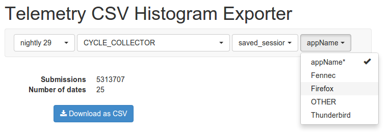
CSV Export with telemetry.jquery.js
One of the really boring and hard-to-get-right parts of the telemetry dashboard is the list of selectors used to filter histograms. Luckily, the user-interface logic for selecting channel, version, measure and applying filters is implemented as a reusable jQuery widget called telemetry.jquery.js. There’s no dependency on jQuery UI, just jquery.ui.widget.js which contains the jQuery widget factory. This library makes it very easy to write a custom dashboard if you just want write the part that presents a filtered histogram.
The snippet below shows how to create a histogramfilter widget and bind to the histogramfilterchange event, which is fired whenever the selected histogram is changed and loaded. With this setup you don’t need to worry about loading, filtering or maintaining state as the synchronizeStateWithHash option sets the filter-path as window.location.hash. If you want to have multiple instances of the histogramfilter widget, you might want to disable the synchronizeStateWithHash option, and read the state directly instead, see jQuery stateful plugins tutorial for how to get/set a option like state dynamically.
Telemetry.init(function(){
// Create histogram-filter from jquery.telemetry.js
$('#filters').histogramfilter({// Synchronize selected histogram with window.location.hash
synchronizeStateWithHash:true,// This demo fetches histograms aggregated by build date
evolutionOver:'Builds'});
// Listen for histogram-filter changes
$('#filters').bind('histogramfilterchange',function(event, data){// Check if histogram is loadedif(data.histogram){update(data.histogram);}else{// If data.histogram is null, then we're loading...}});
});
The options for histogramfilter is will documented in the source for telemetry.jquery.js. This file can be found in the telemetry-dashboard repository, but it should be distributed with custom dashboards, as backwards compatibility isn’t a priority for this library. There is a few extra features hidden in telemetry.jquery.js, which let’s you implement custom <select> elements, choose useful defaults, change behavior, limit available histogram kinds and a few other things.
A complete custom dashboard with CSV export, minimal Javascript code and bootstrap styling, as illustrated in the screenshot above, is available at gist.github.com/jonasfj/8280124. You can fork the gist and build your custom dashboards on top of it. Gist like this can be tested using bl.ocks.org. Hence, you can try to gist above at bl.ocks.org/jonasfj/8280124. You can also build custom dashboards by forking the telemetry-dashboard repository, but the code for this dashboard is more complicated and mainly useful if you want to make a small change to the existing dashboard. In this case you can host your custom telemetry-dashboard fork using GitHub Pages, in fact mozilla.github.io/telemetry-dashboard is used as a staging area for telemetry-dashboard development.
A few days ago Mark Reid wrote a post on the Current State of Telemetry Analysis, and as he mentioned in the Performance meeting earlier today we’re still working on better tooling for analyzing telemetry logs. Lately, I’ve been working on tooling to analyze telemetry logs using a pool of Amazon EC2 Spot instances (tl;dr spot instance are cheaper, but may be terminated by Amazon). So far the spot based analysis framework have been deployed to generate and maintain the telemetry dashboard (hosted at telemetry.mozilla.org). I still need to create a few helper scripts, write documentation and offer an accessible way to submit new jobs, but I hope that the general developer will be able to write and submit analysis jobs in a few weeks. Don’t worry I’ll probably do another blog post when this becomes readily available.
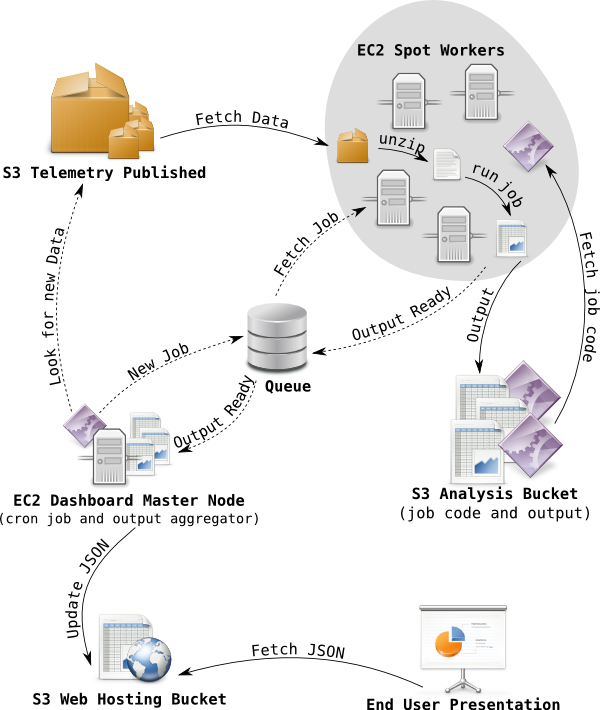
If you’re wondering how telemetry logs end up in the cloud, take a look at Mark Reids fancy diagram in the Final Countdown. Inspired by this I decided that I too needed a fancy diagram to show how the histogram aggregations for telemetry dashboard is generated. Telemetry logs are stored in an S3 bucket in LZMA compressed blocks of at most 500 MB, the files are organized in folders by reason, application, channel, version, build date, submission date, so in practice there is a lot of small files too.
To aggregate histograms across all of these blocks of telemetry logs, the dashboard master node creates a series of jobs. Each job has a list of files from S3 to process and a pointer to code to use for processing. The jobs are pushed a queue (currently SQS) from where an auto-scaling pool of spot instances fetches jobs. When a spot worker has fetched a job it downloads the associated analysis code from a special analysis bucket, it then proceeds to download the blocks of telemetry log listed in the job, and process with the analysis code. When a spot worker completes a job, it uploads the output from the analysis code to special analysis bucket, and push an output ready message to a queue.
In the next step, the dashboard master node fetchs output ready messages from the queue, downloads the output generated by the spot worker, uses it to update the JSON histogram aggregates stored in web hosting bucket used for telemetry dashboard. From here telmetry.mozilla.org fetches the histogram aggregations and presents them to the user. The fancy diagram, below outlines the flow, dashed arrows indicates messaging and not data transfer.
As I briefly mentioned, EC2 spot instances may be terminated by Amazon at any time, that’s why they are cheaper (approximately 20% of on-demand price). To avoid data loss the queue will retain messages after they’ve been fetched and requires messages to be deleted explicitly once processed, of the message isn’t deleted before some timeout, the message will be inserted back into the queue again. So if a spot instance gets terminated, the job will be reprocessed by another worker after the timeout.
By the way, did I mention that this framework processed one months telemetry logs, about 2 TB of LZMA compressed telemetry logs (approx. 20 TB uncompressed), in about 6 hours with 50 machines costing approximately 25 USD. So time and price wise it will be feasible to run an analysis job for a years worth of telemetry logs. The only problem I ran into with the dashboard is the fact that this resulted in 10,000 jobs, and each job created an output that the dashboard master node had to consume. The solution was to temporarily throw more hardware at the problem and run the output aggregation on my laptop. The dashboard master node is an m1.small EC2 node and it can easily keep up with day to day operations, as aggregation of one day only requires 500 jobs.
Anyways, you can look forward to the framework becoming more available in the coming weeks, so analyzing a few TB of telemetry logs will be very fast. In the mean time, checkout the telemetry dashboard at telemetry.mozilla.org, it has data since October 1st. I’ll probably get around to do a post on dashboard customization and aggregate consumption later, for those who would like to play the raw histogram aggregates beneath the current dashboard.
A couple of weeks I introducedTriLite, an Sqlite extension for fast string matching. TriLite is still very much under active development and not ready for general purpose use. But over the past few weeks I’ve integrated TriLite into DXR, the source code indexing tool I’ve been working on during my internship at Mozilla. So it’s now possible to search mozilla-central using regular expressions, for an example regexp:/(?i)bug\s+#?[0-9]+/ to find references to bugs.
For those interested, I did my end-of-internship presentation of DXR last Thursday, it’s currently available on air.mozilla.org (I’m third on the list, also posted below). I didn’t reharse it very much so appoligies if it’s doesn’t make any sense. What does make sense however, is that fact that dxr.allizom.org supports substring and regular expression searches, so fast that we can facilitate incremental search.
(My end-of-internship presentation, slides available here)
Anyways, as you might have guessed from the fact that I gave an end-of-internship presentation, my internship is coming to an end. I’ll be flying home to Denmark next Saturday to finish my masters. But I’ll probably continue to actively develop TriLite and make sure this project reaches a level where it can be reused by others. I’ve already seen other suggestions for where substring search could be useful.
The past two weeks I’ve been working on regular expression matching for DXR. For those who doesn’t know it, DXR is the source code cross referencing tool I’m working on during my internship at Mozilla. The idea is to make DXR faster than grep and support full featured regular expressions, such that it can eventually replace MXR. The current search feature in DXR uses the FTS (Full Text Search) extension for Sqlite, with a specialized tokenizer. However, even with this specialized tokenizer DXR can’t do efficient substring matching, nor is there any way to accelerate regular expression matching. Which essentially means DXR can’t support these features, because full table scans are too slow on a server that serves many users. So to facilitate fast string matching and allow restriction on other conditions (ie. table joins), I’ve decided to write an Sqlite extension.
Introducing TriLite, an inverted trigram index for fast string matching in Sqlite. Given a text, a trigram is a substring of 3 characters, the inverted index maps from each trigram to a list of document ids containing the trigram. When evaluating a query for documents with a given substring, trigrams are extracted from the desired substring, and for each such trigram a list of document ids is fetched. Document ids present in all lists are then fetched and tested for the substring, this reduces the number of documents that needs to fetched and tested for the substring. The approach is pretty much How Google Code Search Worked. In fact, TriLite uses re2 a regular expression engine written by the guy who wrote Google Code search.
TriLite is very much a work in progress, currently, it supports insertion and queries using substring and regular expression matching, updates and deletes haven’t been implemented yet. Anyways, compared to the inverted index structure used in the FTS extension, TriLite has a fairly naive implementation, that doesn’t try to provide a decent amortized complexity for insertion. This means that insertion can be rather slow, but maybe I’ll get around to try and do something about that later.
Nevertheless, with the database in memory I’ve been greping over the 60.000 files in mozilla-central in about 30ms. With an index overhead of 80MiB for the 390MiB text in mozilla-central, the somewhat naive inverted index implementation employed in TriLite seems pretty good. For DXR we have a static database so insertion time is not really an issue, as the indexing is done on an offline build server.
As the github page says, TriLite is no where near ready for use by anybody other than me. I’m currently working to deploy a test version of DXR with TriLite for substring and regular expression matching. Something I’m very much hoping to achieve before the end of my internship at Mozilla. So stay tuned, a blog post will follow…
This year I’m spending my summer vacation interning at the Mozilla office in Toronto. The past month I’ve been working on DXR, a source code indexing and cross referencing application. So far I’ve worked to deploy DXR on Mozilla infrastructure and is happy to report that dxr.mozilla.org is no longer redirecting to dxr.lanedo.com. The releng team have a build bot indexing mozilla-central, so that we always have a fresh index on dxr.mozilla.org. So in blind faith that this will never crash horribly, I’ll tell to:
Whilst I’ve been handling most of the deployment issues, the releng team have been doing the heavy lifting when comes to automatic build, thanks! This means, that I’ve been working on cleaning up, refactoring, redesigning and rewriting parts of DXR. This sounds like a lot of behind the scenes work that nobody will ever see, however, this means that DXR now has a decent template system. And well, who would I be if I didn’t write a template for it.
You can find the tip of DXR that I’m working on at dxr.allizom.org, please check out it and let me know if there’s something you don’t like and would like to appear. I realize that the site currently have a few crashes, and don’t worry I won’t rush this into production before I’ve ratted these out. Now, as evident from this blog, I’m by no means a talented designer, so if you feel that grey should be red or whatever, please leave a color code in the comments and I’ll try it out.
I’m currently looking into replacing the full text search and my somewhat buggy text tokenizer with a trigram index that’ll facilitate proper substring matching and if we lucky regular expression matching. But I guess we will have to wait and see how that turns out. In the mean time leave a comment if you have questions, requests, suggestions and/or outcries.